In this article, I will show how a mathematically simple formula can be used as STRAVA’s GAP (Grade Adjusted Pace) for your runs on a hilly terrain.
In specific, this article provides:
- an Introduction to STRAVA’s GAP;
- Methods for estimating GAP with a formula (see Examples and conclusions);
- Results as well as a validation of the formula against real data from STRAVA;
- some food for thought and Discussion;
- data and code to reproduce and extend the results, and for estimating and analysing the GAP from a spreadsheet (download here) or a .fit file (download here);
- my hopes that it will help, appended with the References!
Introduction to STRAVA’s GAP
Running uphills or downhills is expected to require different effort than running on flat terrain at equal pace. To facilitate the comparison of running efforts or paces on different elevation grades (Lloyd, 2013), STRAVA has invented a metric called Grade Adjusted Pace (GAP). Given a pace on a specific grade (positive value for uphills, and negative for downhills), GAP is the pace you would run at equal heart rate on flat ground (Robb, 2017). Presumably, STRAVA calculates GAP point estimates based on an activity’s course point measurements of elevation and pace uploaded by a subscribed user only (it was free until May 2020; see Smith, 2020). The point-wise nature of estimation is inferred by the replies to the post of Reddit user “kovasin” (2014) by user “therealslloyd” who appears to be a developer of STRAVA’s GAP (Lloyd, 2013). Upon uploading the activity, the company provides (Rosie, 2021):
- two plots of GAP across the course:
- a lineplot, presumably over GAP point estimates;
- a barplot of GAP split estimates, presumably the mean GAP from the 1.a point estimates of each split;
- a table with the GAP split estimates of 1.b which can be copied as text;
- the mean GAP over the entire course.
Note that the GAP point estimates by STRAVA in 1.a cannot be copied or exported in any automatic way, and there are seemingly two ways we can extract GAP values of lower resolution or quality. First, the highest resolution of GAP values you can get can only be accessed manually, i.e. by hovering over the related graph. Moreover, we can access only four to five GAP values from consecutive course points per 100 m, testing our eyes and hand in moving the mouse cursor pixel-by-pixel on screen (the author had to configure the computer to be able to move the cursor pixel-by-pixel via the keyboard). Due again to STRAVA’s not fully transparent methods, we cannot know whether these “hovering” GAP values are indeed point estimates (at the highest resolution in which STRAVA calculates GAP), or they are k-nearest-neighbour summaries of elevation, pace or GAP. Second, we can extract the GAP values from the lineplot of 1.a. A screenshot of the graph can be fed to a tool such as the WebPlotDigitizer (Rohatgi, 2021), which returns x–y coordinates after manually calibrating the screenshot’s axes. Given all this inconvenience, many users have still wondered if there is any way to automatically download all GAP point estimates from a course (e.g. see post by Reddit user “conspatz”, 2020). Typical responses, as the one to the latter post, are negative, advising to calculate GAP from the point measurements of elevation and pace, although they “don’t know the formula by heart, but should be pretty easy to Google it”.
Nevertheless, it appears that the GAP formula is not at all pretty easy to find, no matter how much we Google it. Many people have hence kept looking, with feelings ranging from mere confusion of recreational runners (e.g. see post of Reddit user “kovasin”, 2014), to complete frustration of developers (e.g. see post of Reddit user “ttraxx”, 2019). The only reliable information about the inner workings of STRAVA’s GAP estimation is provided in two posts by people who have developed it. In the first post, Lloyd (2013) explains the motivation behind GAP, the previous scientific works which inspired GAP, and how it was improved in the newer version. The few clues are provided only verbally. For example, Lloyd (2013) explains that GAP is faster on steeper uphill running, slower on steeper downhill running, but running downhill on grade higher than −20% does not lead to higher GAP. Moreover, it is mentioned that these adjustments are not quantities independently added/subtracted as in the previous GAP implementation; they are rather proportional to the hill pace. In the second post, Robb (2017) elucidates further the form of this newer GAP model by including a plot which depicts the empirical data it was fitted on (Fig. 1 herein).
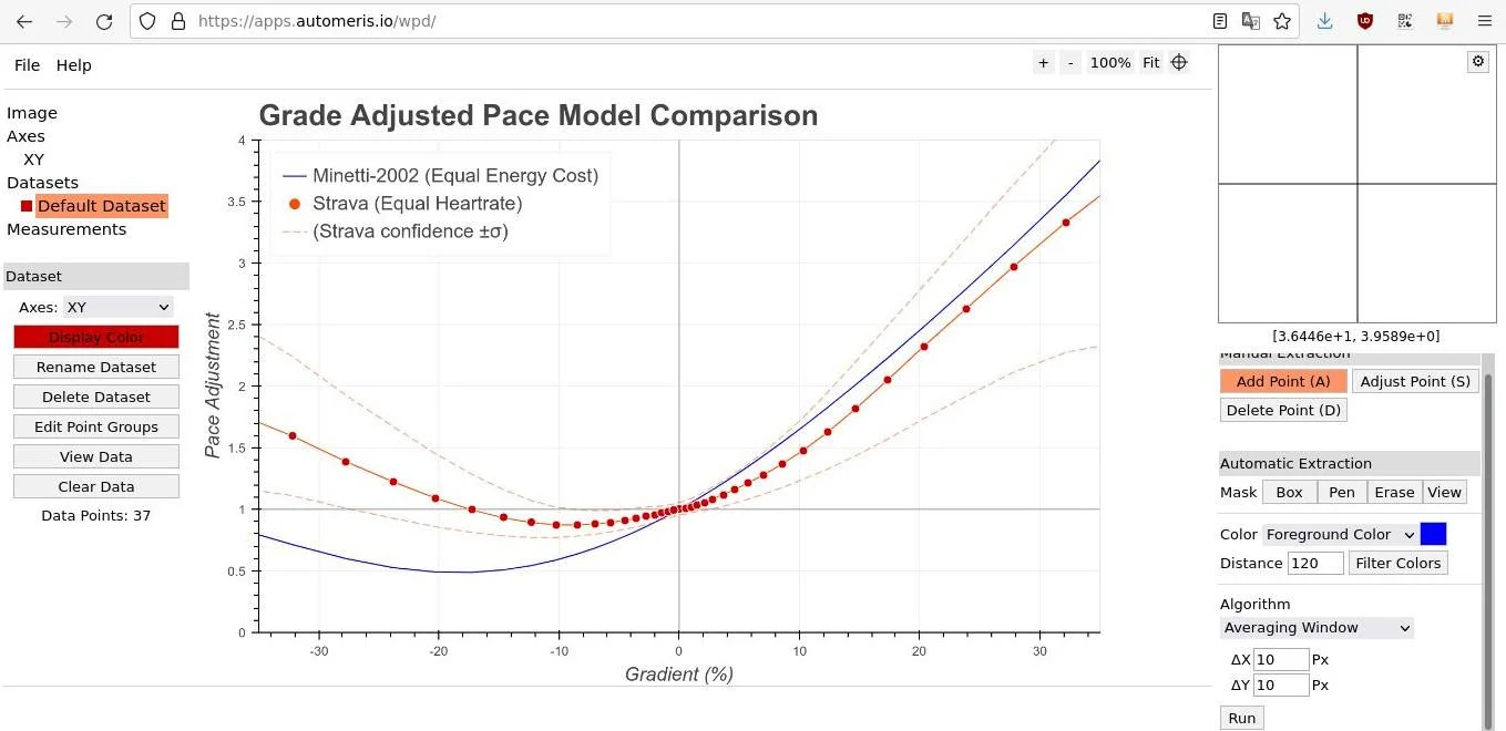
From what I understand based on the brief descriptions in the two aforementioned posts, the plot with the STRAVA empirical data points has the grade g at the x-axis, whereas the y-axis represents a hereafter called adjustment coefficient a(g) (Fig. 1). STRAVA’s model hence establishes a relation for the adjustment coefficient a as a function of the grade g. “Pace adjustment” on the plot’s y-axis refers to the pace on flat ground, F. By multiplying F with a related via the model’s curve to a specific grade g, we estimate what the hill pace H would be with equal heart rate if we were running at that specific grade. That is, H = a(g) · F. Confirming the information provided by Lloyd (2013) and Robb (2017), STRAVA’s fitted model in Fig. 1 predicts for a > 1 a slower pace on steeper than around −20% downhill terrain and when moving uphill for a given pace on flat terrain, and for a < 1 a higher pace on less steeper downhill terrain. According to the definition of GAP in the Introduction though, we are commonly faced with the reverse situation of a hill pace for which we want the effort-equivalent flat pace, i.e. the GAP = F = H / a(g), after rearranging the last equation. Thus, although the model links the adjustment coefficient a to the grade g, GAP is obtained via the reciprocal of a. In other words, by multiplying the hill pace with the 1 / a(g) related to the specific grade g, we obtain an estimate of what the pace would be with equal heart rate if running on flat ground. Nevertheless, the formula or at least the type of the fitted model are not provided, to facilitate the understanding and usage of GAP by other users.
The present work aimed to help such users by providing a formula for estimating a GAP hopefully similar to STRAVA’s. The formula’s derivation is based on the only quantitative clues available for their GAP model, i.e. the plot in Robb (2017). The data point coordinates extracted from the plot are used for fitting appropriate models which are also simple and mathematically representable with equations, to facilitate sharing and usage. The best and most plausible among the models is then tested against a running activity I did specifically for this purpose, to test if the present work’s GAP estimates are close to the values provided by STRAVA (I subscribed for one month free).
Methods
To facilitate the transparency, reproduction and extension of the present work, all data, analyses and plots can be downloaded from here. All analyses and plotting were carried out in R (R Core Team, 2020). In specific, the following R packages were employed:
- tidyverse for data processing and plotting (Wickham et al., 2019);
- patchwork for plot insets (Pedersen, 2020);
- lubricate for transforming paces to seconds and vice versa (Grolemund and Wickham, 2011);
- FITfileR for processing .fit activity files from my device (Smith, 2022);
- xts for working with time series (Ryan and Ulrich, 2020);
- forecast for smoothing time series out (Hyndman et al., 2020).
Extracting STRAVA’s empirical data for fitting the models
Brief information about the point-binned empirical data depicted in the plot of Fig. 1 can be found in Robb (2017). The extraction of the data point coordinates was done online with WebPlotDigitizer (Rohatgi, 2021).
Fitting the models
Given the positioning of the data points on the a–g plane (Fig. 1), polynomial models seemed appropriate. Moreover, such models are simple, but also easy to share and use by the values of the model coefficients. I tried five polynomial models of increasing order: from 2nd- to 6th-order. For example, the 2nd-order polynomial model was of the form: a(g) = Intercept · g0 + A · g + B · g2, where the Intercept, A and B are model coefficients taking real values such that the model’s curve should have the best but also most plausible fit.
Theoretically, we expect that when the grade g equals 0%, there is no need to adjust the pace, i.e. the pace adjustment coefficient a(0) must equal one, to lead to no adjustment after multiplication with the pace: H = a(0) · F = 1 · F = F. Hence, all polynomial models in the present work were forced during fitting to pass through point a(0) = 1, i.e. to have an intercept equal to one. This was done via Weighted Least Squares. Keeping in mind the inherent error in the extraction of STRAVA’s data point coordinates as from the plot in Fig. 1, the extracted data point closest to the expected a(0) = 1 had coordinates a(0.9944) = 1.0167. Thus, I had to add another data point which had gradient equal to 0% and adjustment coefficient equal to one. This data point was then given a fitting weight adequately higher than the rest of the data points.
Validating the best-performing model with a test case
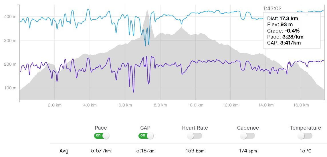
The test case was from a run I did specifically for the purpose of validating the best-performing model of this work. I took the first-month-free STRAVA subscription to obtain their GAP data for my run (Fig. 2). For the validation, I used two sources of GAP data. First, the table which STRAVA provides with presumably each split’s mean GAP of its point estimates. I tested if indeed the table values are averages of GAP point estimates of each split. Second, I extracted GAP-versus-distance data from the lineplot of Fig. 2 with the WebPlotDigitizer (Rohatgi, 2021). This online tool implements algorithms for extracting automatically points based on the line’s colour.
I specifically chose this course for its diversity of grades, to challenge the present work’s model under a variety of conditions. Additionally, I ran it with an as much as possible wider range of grade-versus-pace combinations. For example, parts of the steep side at the 8th km were passed by either running as fast as I could or by walking, both during the ascent and descent. Finally, I tried to run some segments with stable heart rate, or stable perceived effort of standing comfortably upright under the lactate ceiling (e.g. see pace and GAP values at the 9th and 11th–12th km in Fig. 2). Note that the aim of this validation exercise is to test whether a fitted polynomial returns GAP values close to STRAVA’s, and not to test whether any model provides good predictions for different users or conditions. This is the reason I did not employ other activities or users for this validation test. If STRAVA’s model is a formula-like, fixed one—and independent of other user-specific variables such as heart rate, weather or terrain technicality—then a single activity with high enough variability in grade and pace, such as the present test case, should be enough to reveal any model disagreement.
The selection of the best-performing model was based on its plausibility, on its ability to extrapolate to extreme values of grade and pace, and on the coefficient of determination R2 when fitted on STRAVA’s empirical data as of Fig. 1. The ability to extrapolate beyond the range of the empirical data is very important, because STRAVA’s model appears to be fitted to empirical data in a grade range of around ±30% (Fig. 1), but we can find grades of higher magnitude in real. The R2 metric ranges from zero to one, with higher values indicating a model with better fit, and hence of higher agreement with STRAVA’s model which is tightly overfitted to the empirical data points (Fig. 1).
Results & Discussion
The fitted polynomial models
Only the polynomials of 2nd- and 3rd-order behaved well on STRAVA’s empirical data, and beyond (Fig. 3). According to the inset, only these two models predicted an adjustment coefficient which was always above zero for grades beyond the range they were fitted on, as expected. In specific, a negative adjustment coefficient makes no sense, because it would lead to a negative flat pace (and to a negative hill pace, when using the coefficient’s reciprocal for estimating GAP). Additionally, the trend in these two models is desirably increasing mildly for both more negative and more positive grades. The behaviour of the model is very important to be taken into account, especially for more extreme values of the input variables than the ones the model was fitted on. For example, GitHub user “ElsitaK” (2020) has fitted a 4th-order polynomial model similarly on the empirical data of STRAVA, but we have herein seen that this polynomial returns negative values for sufficiently higher uphill grades than the ones of the empirical data (third in darkness curve in the inset of Fig. 3).
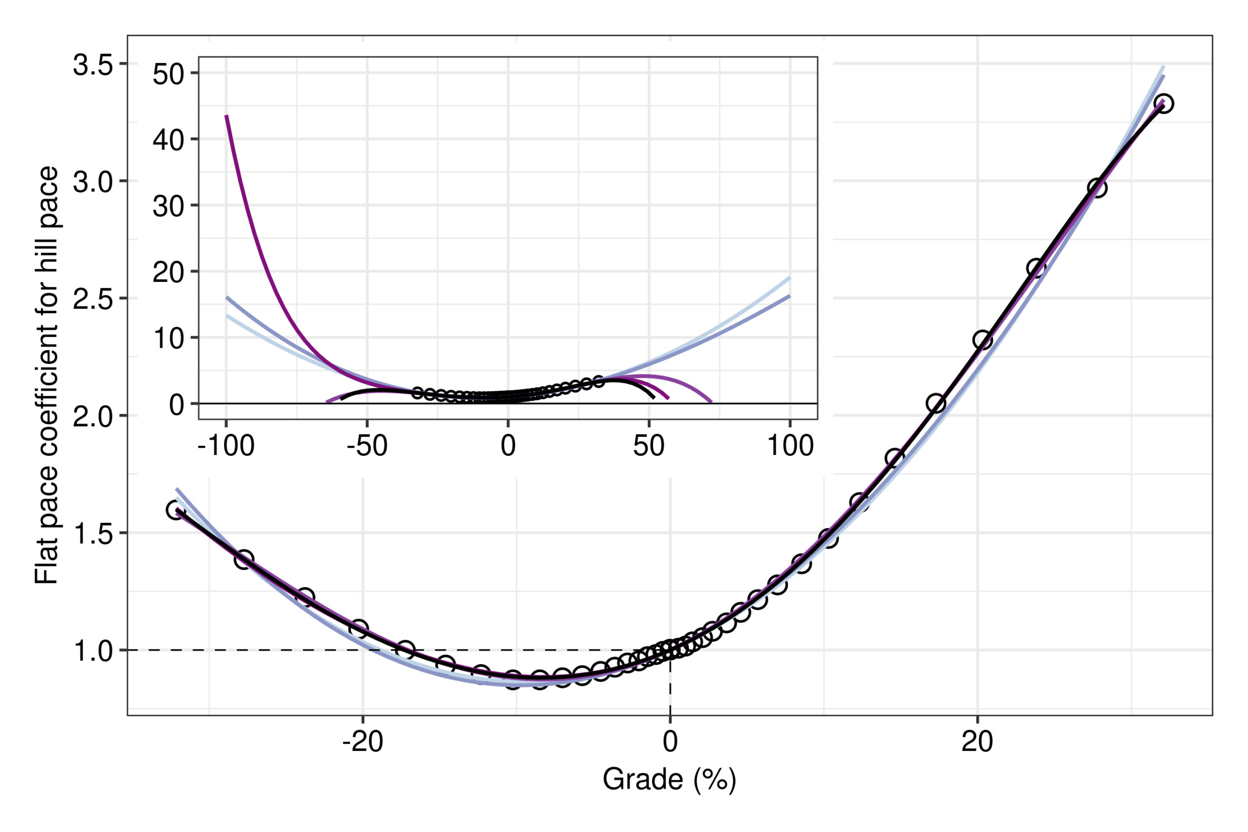
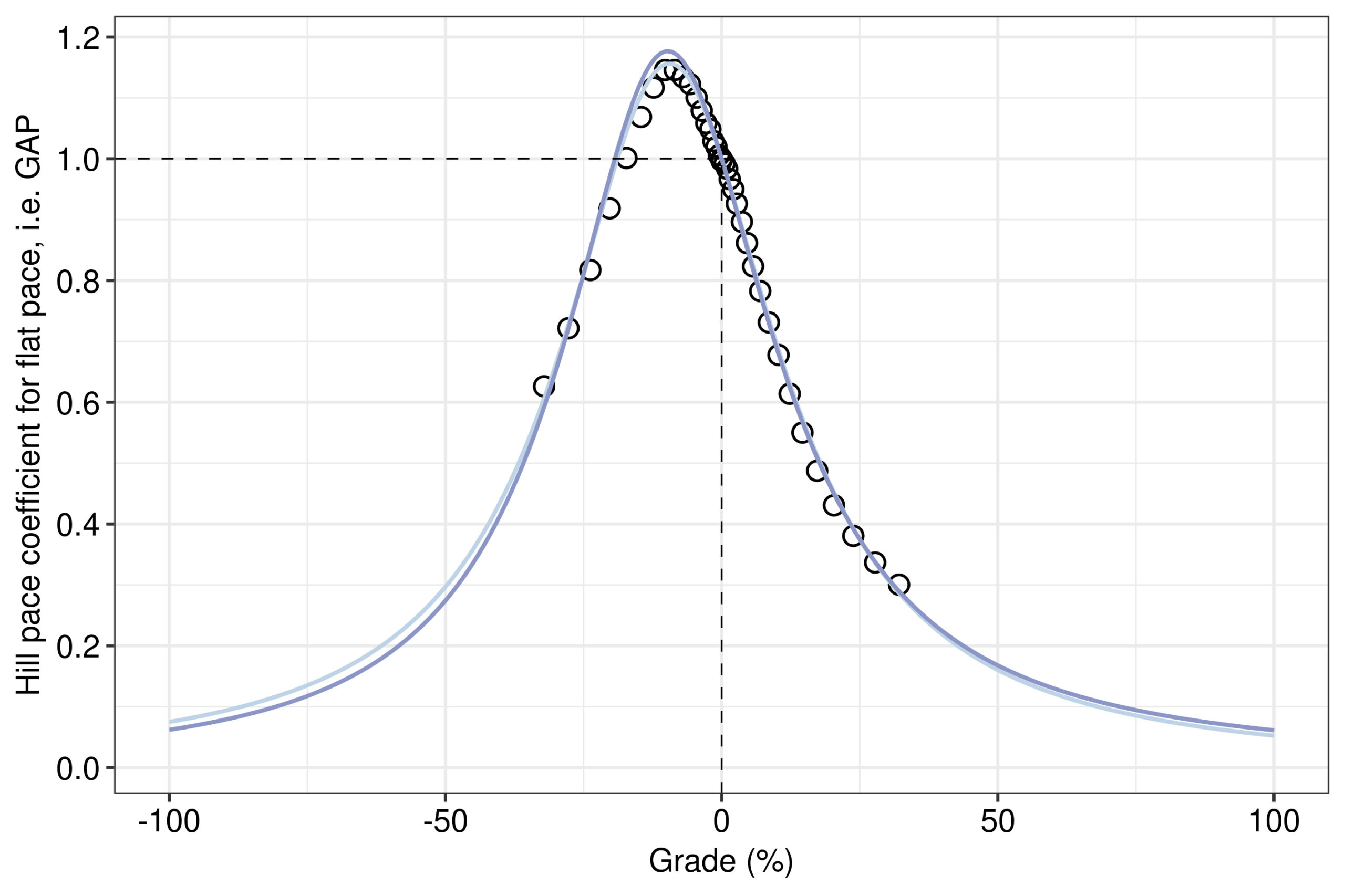
The model coefficients of the two well-behaved polynomials of 2nd- and 3rd-order are given at a precision of six significant digits in Table 1. At this precision, their intercepts are desirably equal to one. Both polynomial models exhibited a very good fit, with a coefficient of determination R2 of 0.9957 and 0.9961 for the 2nd- and 3rd-order, respectively. Despite having a slightly lower R2, the 2nd-order polynomial’s fit was more satisfactory. This was more apparent when looking at the reciprocal of a at the y-axis, which is the coefficient by which the hill pace is multiplied at a specific grade to obtain the flat-equivalent GAP (Fig. 4).
|
Grade |
2nd-order model’s |
3rd-order model’s |
|---|---|---|
| g0 | 1.000000E+00 | 1.000000E+00 |
| g1 | 2.869556E-02 | 3.052871e-02 |
| g2 | 1.520768E-03 | 1.520751e-03 |
| g3 | – | −2.954431e-06 |
In specific, the 2nd-order polynomial’s reciprocal of the adjustment coefficient, 1 / a(g), passed closer than the 3rd-order polynomial from STRAVA’s empirical points at the important region of downhill grades of around –10%, where GAP reaches its maximum for a given pace (Fig. 4). Perhaps, the fit would be even better at this important region between 0% and –20% grade, where GAP is higher than the actual pace, if STRAVA’s empirical data points were more smoothly aligned around g = 0%. An additional constraint to the fitting arose because the models were forced to pass through point a(0) = 1. Nevertheless, the present work provided a limited range of models just for illustration with some simple but robust and easy-to-share models. Given the data point coordinates extracted as in Fig. 1, it would be straightforward to fit other models of much higher flexibility, e.g. LOESS, although they are commonly difficult to represent with a mathematical formula. The lack of a mathematical formula for GAP would be a limiting factor when developing applications in environments which cannot process more elaborate models.
The test-case validation of the best polynomial model against STRAVA’s GAP
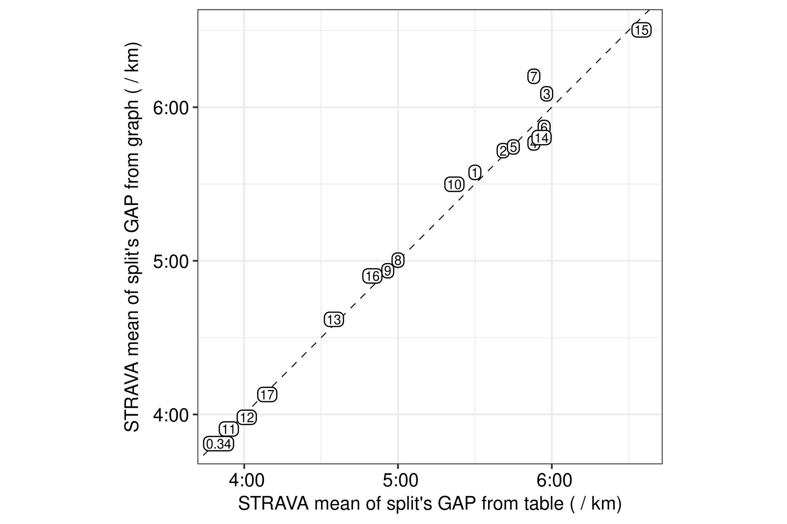
The first thing I tested was whether STRAVA’s GAP for each split which is provided in the test case’s activity board was indeed a mean of GAP point estimates. The GAP point estimates were assumed to be the ones in the GAP lineplot provided by STRAVA (Fig. 2). Of course, the lineplot could provide only a visually smooth and less noisy summary of the point measurement data, although STRAVA could be using the raw point values for calculating the GAP means of each split. Nevertheless, in the case of a good agreement, then there is a good chance that both the lineplot displays the actual data used for the calculations, and that the split GAP values in the tables are indeed means from each split’s GAP point estimates. Indeed, this was the case, since there was a good agreement between the GAP values of the splits from the table and the means I calculated for each split’s extracted data points from the lineplot (Fig. 5). These results hence confirm that most likely the GAP point estimates which STRAVA works with are indeed the ones shown in their GAP lineplot.
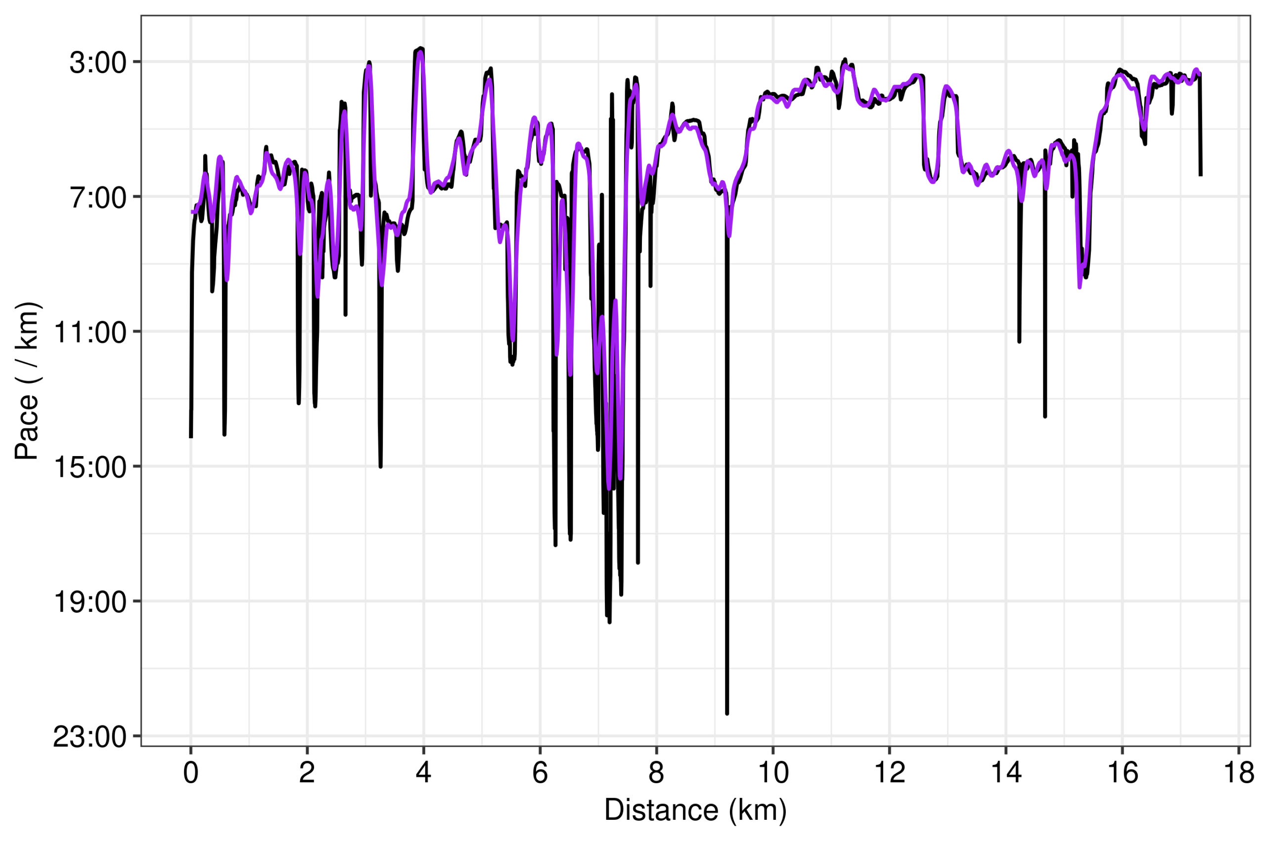
A follow-up question would then be whether the relatively smooth GAP lineplot (Fig. 2), which displays the actual GAP data estimated by STRAVA as we confirmed with Fig. 5, is obtained by the raw measurements of pace and grade uploaded by the user. We can directly test this for pace, because we have access to our own pace data from the device. Indeed, STRAVA’s lineplot for pace is a smooth, heavily denoised and outlier-free version of the raw data (Fig. 6). It also appears that STRAVA has applied considerably more denoising to the lower values of pace.
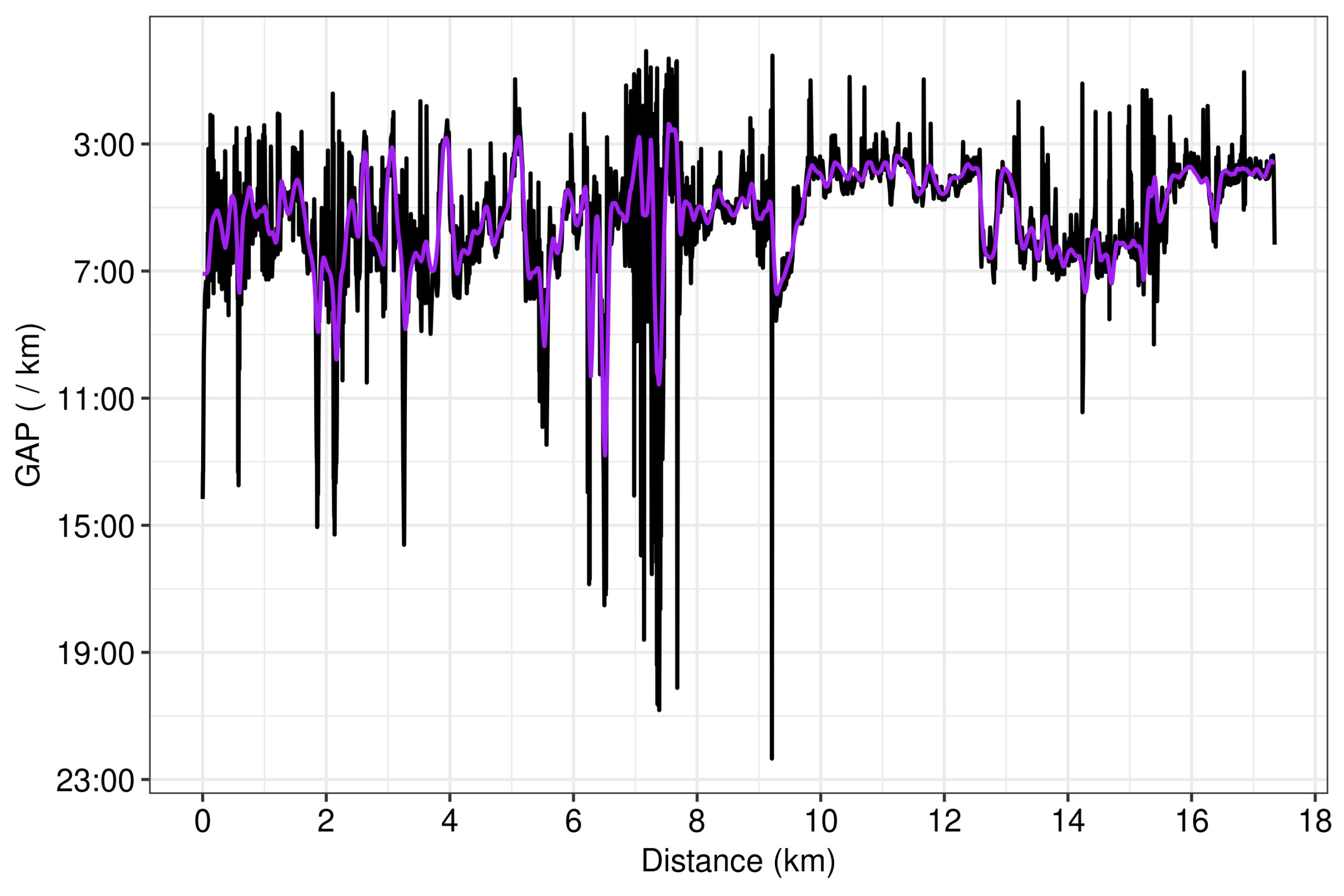
Knowing that GAP comes from the multiplication of pace by a coefficient related to grade (Fig. 4), we can expect that STRAVA uses the smooth version of pace displayed in their lineplot for calculating the similarly smooth GAP lineplot (Fig. 2). We can test this by firstly calculating the GAP for the raw measurements of pace and grade from the device with the 2nd-order polynomial of the present work. Indeed, the polynomial’s GAP from the raw data is much more noisier than STRAVA’s lineplot (Fig. 7).
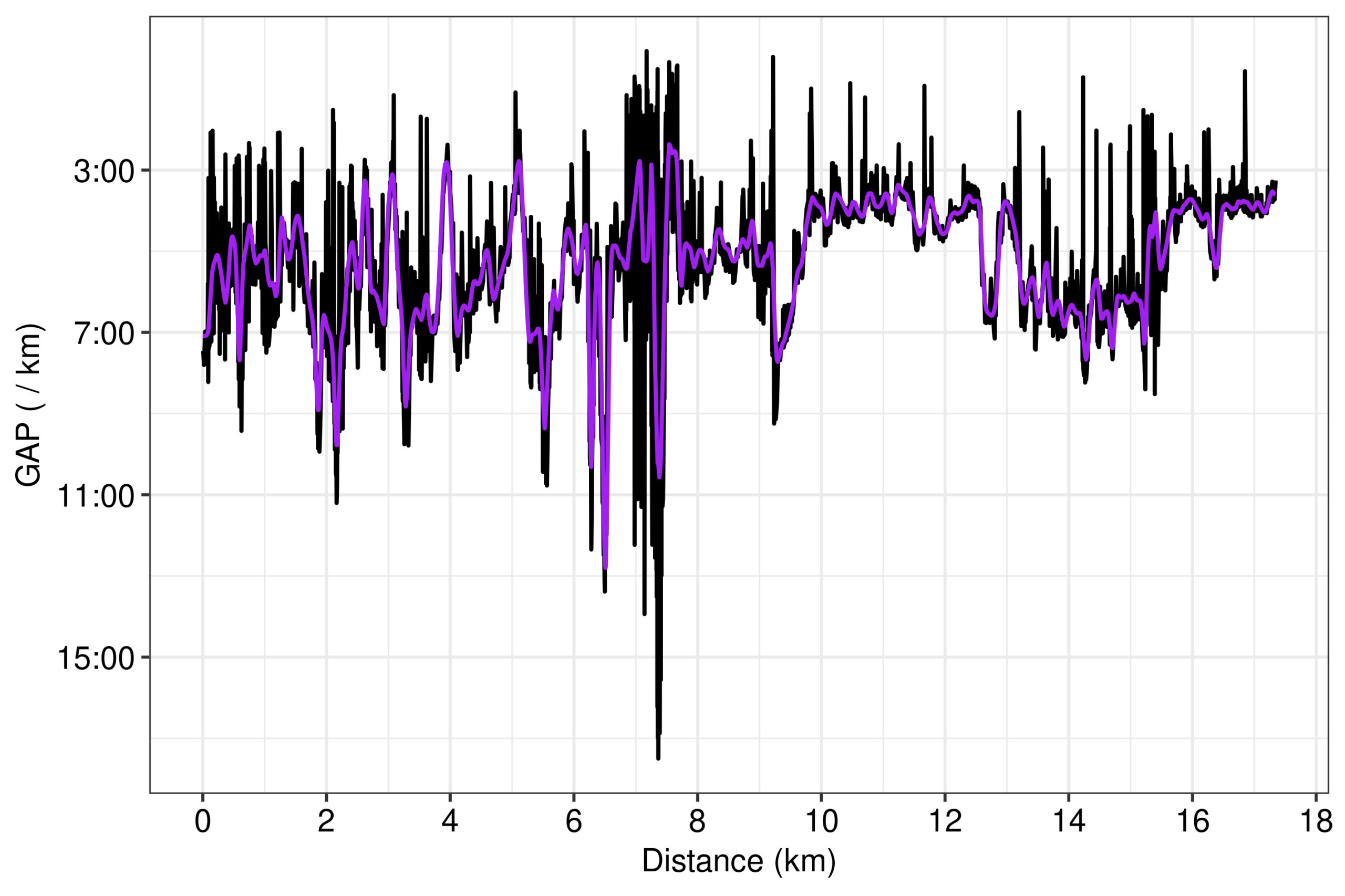
Secondly, we can instead use the smoother pace lineplot data from STRAVA to again calculate GAP with the polynomial model. If the GAP series from the polynomial becomes smoother, it means that most likely STRAVA smooths pace before using it for the GAP calculation. Indeed, the GAP series lost many of its outliers, especially for lower GAP values (Fig. 8). This was expected, since as it was already noted, the main difference between the raw pace and STRAVA’s pace in their lineplot was their cleaning of outliers from the low end of pace (Fig. 6). Still, though, the polynomial GAP is much more noisy than STRAVA’s, which naturally leads to our final attempt to smooth GAP: by smoothing the second constituent component of GAP, i.e. the grade.
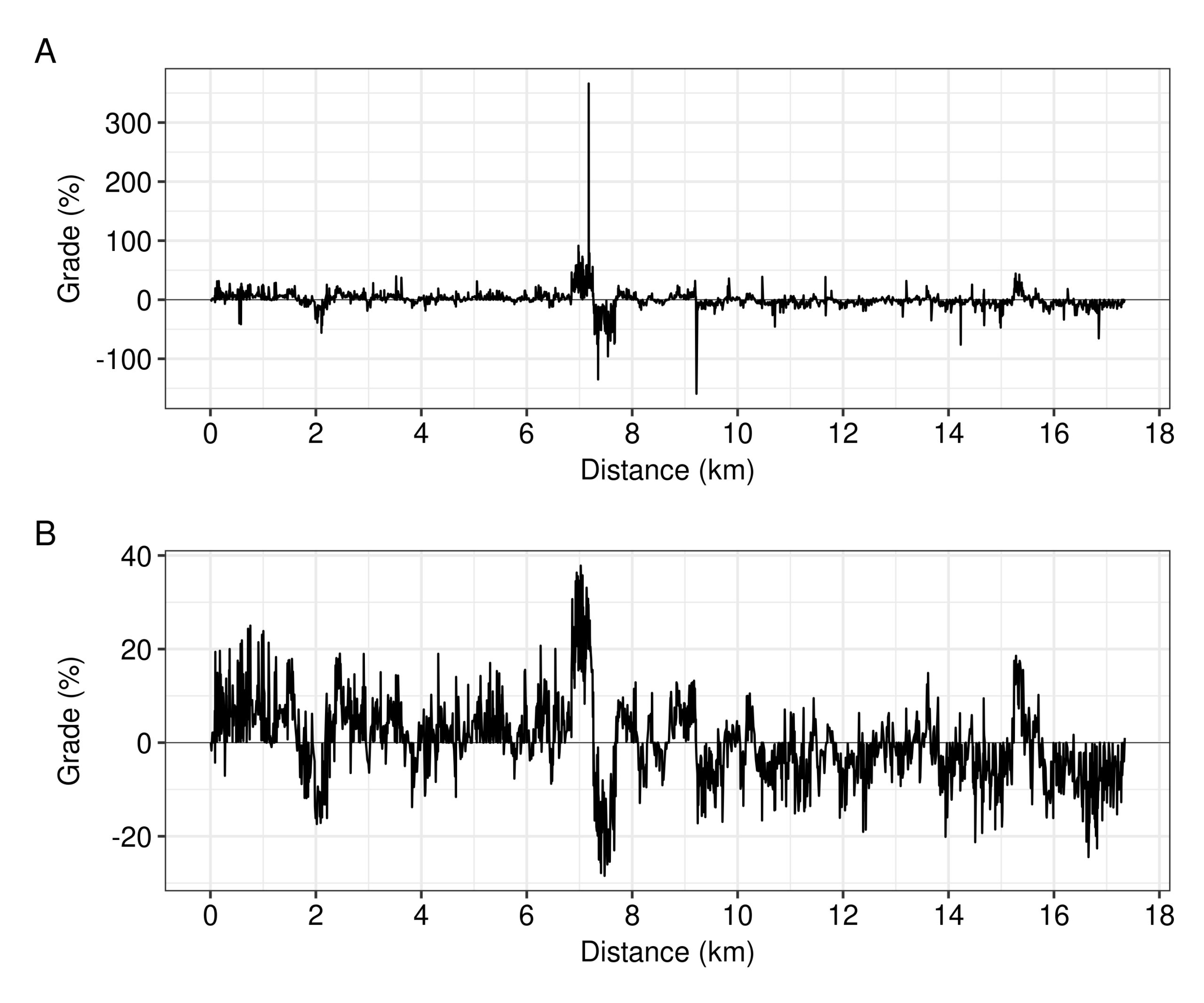
Thirdly, then, we can try to remove the outliers from the raw grade measurements of the device (Fig. 9A). The grade series of my activity includes some extreme and unrealistic values (e.g. 300%+ at the 8th km). The identification of outliers can be based on different extent limits. For example, a common criterion for identifying a data point as an outlier is if it is further away than k = 1.5 times the interquartile range of the data points. Since we don’t know anything about how STRAVA identifies outliers and smooths a series, the strategy was to attempt outlier removal and smoothing of the grade series for different values of k, then to calculate GAP with the polynomial model for the processed grade series (and the smooth pace series from STRAVA’s lineplot), and finally to calculate the mean distance between the calculated GAP series and the smooth GAP series from STRAVA’s lineplot. Thus, the smoothing of the grade series which minimised the dissimilarity between the two GAP series was when k = 1.6. This finally selected grade series lacked the unrealistically extreme values of the raw grade series (Fig. 9B). Although the selected grade series had some flows, e.g. the profile of the steep hillside at the 8th km which I ascended and immediately after descended was not very symmetrical, I believe it was a reasonable approach to follow, given the absence of any information about how the company smooths their series out.
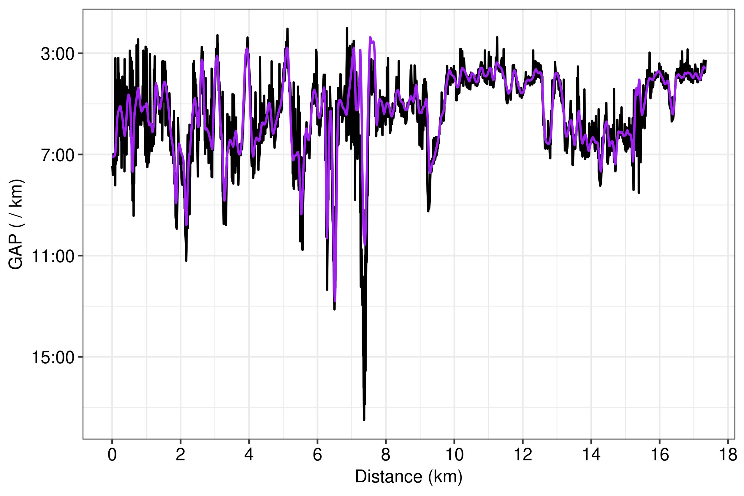
Finally, the GAP series calculated by the 2nd-order polynomial with the smooth pace lineplot data of STRAVA and the smoothed grade data was much more similar to STRAVA’s GAP lineplot (Fig. 10). Of course, their GAP series is even more smooth, but I decided to not invest more time in smoothing the polynomial GAP series further. Besides, the polynomial GAP series had noise equally above and below STRAVA’s GAP series, except in some particular course parts, such as in that steep hillside at kilometre 8. The point is that if the noise of the polynomial GAP series is uniformly spread above and below STRAVA’s GAP series, then I would expect that the means for the GAP of each split between the two methods would not disagree considerably. This was the subsequent test undertaken…
Fortunately, the means of the splits’ GAP point estimates with the polynomial model were in close distance to the split GAP means from STRAVA’s table (Fig. 11). This was good news, because it meant that the present work’s simple quadratic equation can estimate GAP pretty similarly to STRAVA’s hidden model. The means of the polynomial model’s split GAP estimates had a median of around 5 sec distance from STRAVA’s, with the 75% of the means not more than 17 sec apart from STRAVA’s. Additionally, STRAVA provides a mean GAP over the entire activity equal to 5:18 / km, whereas the GAP series from the polynomial model had a mean of 5:26 / km. Only the mean GAP estimate of that split at the 8th km was much further away from STRAVA’s estimate, i.e. estimated 1:40 / km slower pace than STRAVA’s, but we have already noted some clues for the reasons underlying such disagreement. The last investigation of the present work’s lengthy analysis is dedicated to this explanation.
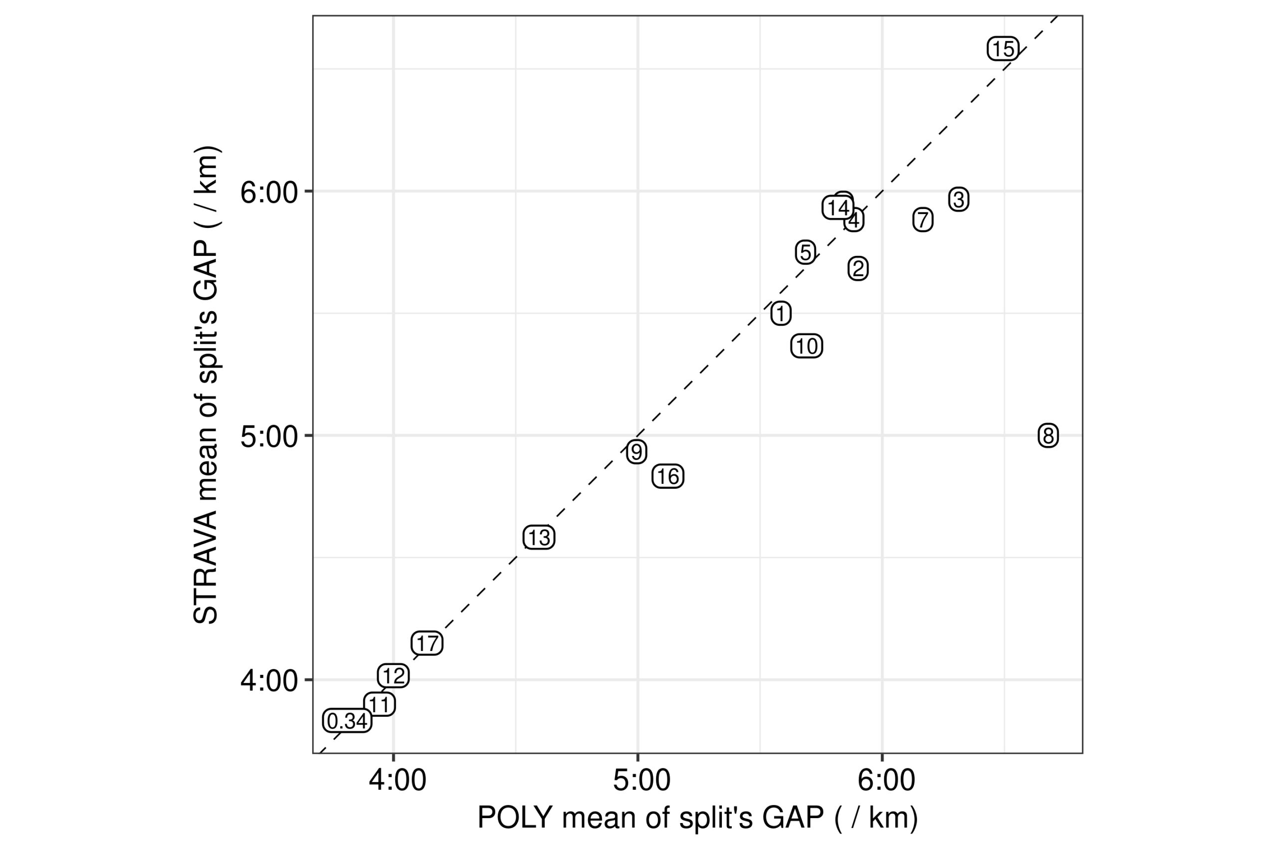
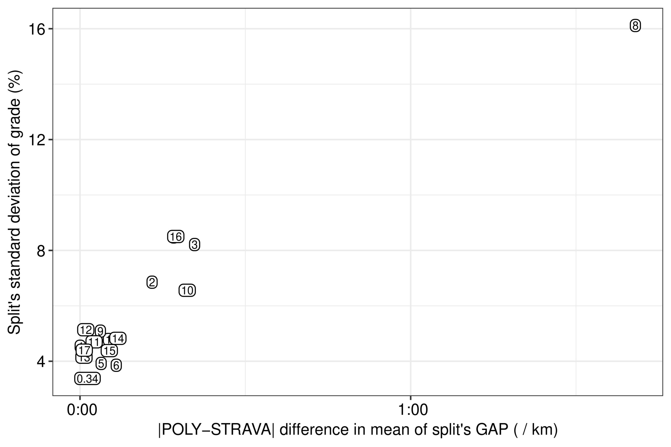
Since we used the smooth pace data from STRAVA’s lineplot for calculating GAP with the polynomial model, only grade could be the source of noise for explaining any disagreement between the two mean GAP estimates for each split (Fig. 11). For example, the greatest discrepancy between the two GAP series was found at the 8th km (Fig. 10). The characteristic difference in our smoothed grade series between that split of steep ascent and descent and the rest of the splits was its higher variation in the grade, e.g. from above 20% to below –20% in just the first half of the kilometre (Fig. 9B). Indeed, the absolute difference between the mean of each split’s GAP from the polynomial model and STRAVA’s mean from the table was positively related to the variation of the split’s grade in the grade series which we smoothed herein (Fig. 12). Thus, any discrepancy of the polynomial-based GAP point estimates can be attributed to the smoothing method used, and not to the present work’s model per se. We could attempt more sophisticated methods for smoothing the grade and pace series, as STRAVA does, but this would go beyond the scope of the present work, the aim of which was to build an equation to satisfactorily approximate STRAVA’s GAP estimates.
Examples and conclusions
The present work showed that a simple model of a quadratic equation can adequately estimate GAP similarly to STRAVA’s method. For two significant digits from Table 1, this 2nd-order polynomial equation is:
a(g) = 1 + 0.029 · g + 0.0015 · g2,
where g is the percent grade, and a(g) is the coefficient by which a flat pace F must be multiplied to estimate the hill pace H at equal heart rate on that specific grade, H = a(g) · F. Note that paces are in the conventional format of minutes per km or mile, and they are converted to seconds per km or mile for the calculations.
Commonly, we want the GAP, which is the F = H / a(g). Thus, given a hill pace H and the grade on that hill, we can feed the quadratic equation with the grade, calculate the value of a(g), and then take the reciprocal of that value, 1 / a(g), and multiply the hill pace H to obtain F, i.e. GAP.
For the examples shown in Fig. 13 (sensu Beatty, 2025), the grades were chosen to be 1% and −1% because it makes the math really easy, and they represent slight uphill/downhill. A flat 0% grade was added to show that F = H when running on level ground. Finally, the 20%, 10%, −10%, and −20% were included to show some extreme slopes (including the crossover point where extreme downhill becomes harder instead of easier than in flat).
The input pace is the same throughout so that it is easier to see how (only) the grade affects the converted paces. Note that using min/mile would return the equivalent GAP values but in the Imperial system.
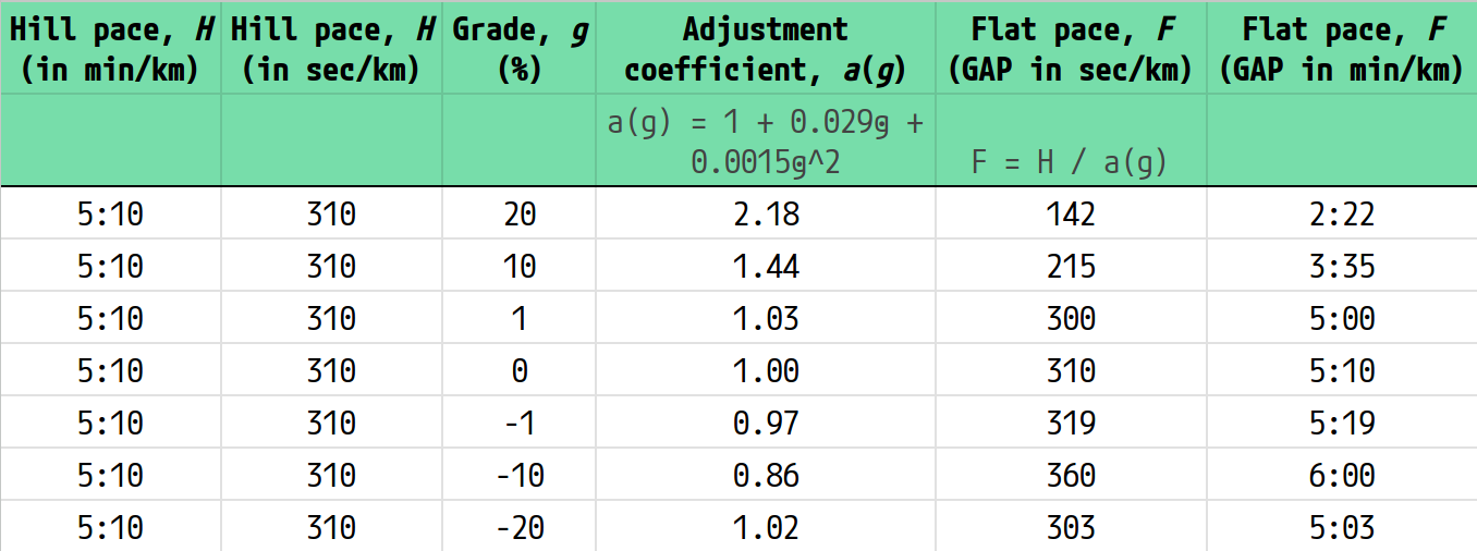
You can use this spreadsheet by downloading it here (.ods format; can be opened by MS Excel and other products).
In conclusion, given the non-transparency of the company’s methods (e.g. about smoothing the pace and grade data before estimating GAP with their fitted model), together with our lack of knowledge about any additional algorithmic rule they might be using on top of the model (e.g. for extreme grades), I believe that the present work’s fitted quadratic model does a pretty decent job in estimating GAP. I hope it will be of help, or at least stimulate some discussion from us outside the [black] box!
Acknowledgements
I would like to thank Doug Beatty for the valuable feedback that improved this article with his provided Examples.
References
Beatty, D. (2025) Illustrative examples and edge cases for the quadratic formula. Personal communication, February 2025.
GitHub user “ElsitaK” (2020) Running_Wild: data manipulation and analysis for “Running Wild” virtual race, fundraiser for Piedmont Wildlife Center.
Grolemund, G., & Wickham, H. (2011). Dates and Times Made Easy with lubridate. Journal of Statistical Software, 40(3), 1-25.
Hyndman, R. J., Athanasopoulos, G., Bergmeir, C., Caceres, G., Chhay, L., O’Hara-Wild, M., … & Wang, E. (2020). Package forecast.
Lloyd, S. (2013) Improving Grade Adjusted Pace. Accessed on January 25, 2022.
R Core Team (2020). R: A language and environment for statistical computing (R version 4.0.2). Computer software, R Foundation for Statistical Computing, Vienna, Austria.
Reddit user “conspatz” (2020) Getting Grade Adjusted Pace via the Strava API. Accessed on January 25, 2022.
Reddit user “kovasin” (2014) GAP is confusing me. Accessed on January 25, 2022.
Reddit user “ttraxx” (2019) Grade Adjusted Pace… WTF is the formula?! Accessed on January 25, 2022.
Robb, D. (2017) An improved GAP model. Accessed on January 25, 2022.
Rohatgi, A. (2021) Webplotdigitizer: Version 4.5.
Rosie (2021) Grade Adjusted Pace (GAP). Accessed on January 25, 2022.
Ryan, J. A., & Ulrich, J. M. (2020). xts: eXtensible Time Series. R package version 0.12.1.
Pedersen, T. L. (2020). patchwork: The Composer of Plots. R package version 1.1.1.
Smith A. (2020) Strava moves key features from free to subscription-only. Accessed on January 27, 2022.
Smith, M. (2022). FITfileR: Read FIT files using only native R code. R package version 0.1.4.
Wickham, H., Averick, M., Bryan, J., Chang, W., McGowan, L. D. A., François, R., … & Yutani, H. (2019). Welcome to the Tidyverse. Journal of open source software, 4(43), 1686.
